4 Deep Learning, Large Language Models, and Embeddings

4.1 Introduction

This chapter comprises two sections. First, we discuss the architecture and essential operation of deep learning models. In part two, we present the concepts and vocabulary specific to large language models (LLMs), a particular type of model designed for text generation and analysis.

4.2 Deep Learning Models

Before discussing the operation and architecture of deep learning models, we must first define a model. A model is nothing more than a computational/mathematical representation of reality. Remember that just as a map is not the territory, a model is not reality. That means – in practical terms – that no model perfectly represents reality. Or, as the mathematician George Box put it, “All models are wrong, but some are useful.” Computational models come in all sizes and flavors, but the focus here will be on deep learning models, also known as neural networks.

As its name suggests, neural networks are composed of artificial neurons. In Figure 1, each yellow box is an artificial neuron or node. Each node contains a net input function – pictured here as a plus sign inside a purple circle – and an activation function – pictured as a step inside a light green box. The job of the net input function is simple. Add up all the incoming inputs and pass that value to its activation function, which calculates the node’s output.

The lines between the nodes are essential. These are the model’s adjustable parameters or weights. (Both terms are found in the literature.) The output from each node is multiplied by these weights before entering the downstream node. This is an important point as model weights are adjusted during the training process. This is how a neural network learns. The model training process consists of two overarching phases.

During forward propagation, input features found in the dataset are first fed to the network’s input layer, shown here as X1 and X2. From there, these values are multiplied by the weights that sit between the input nodes and node G, the only node in our hidden layer. Keep in mind that deep learning models only understand numbers. Thus, all training data must be converted to a numeric format before a neural network can digest it.

The movement of numbers is from left to right during forward propagation. In this example, the final node – node F – outputs the model’s prediction, otherwise known as its inference. That value is then passed to an error (loss) function, which calculates the difference between the model’s prediction and ground truth, the correct or expected answer.

During backpropagation (backprop), the flow of numbers reverses itself, moving from right to left. As the optimizer adjusts the model’s weights, it learns the underlying patterns found in the data. The forward and back propagation cycle continues until the model hopefully converges to a final state where its inferences are almost always correct. The minor adjustments to the weights during each training cycle (epoch) are made in relation to each one’s contribution to the model’s total error. Trained models can do many interesting things, as we see next.

4.3 Large Language Models

Large language models (LLMs) are a special kind of deep learning model that can create word embeddings. Word embeddings lie at the heart of natural language processing (NLP), enabling systems like ChatGPT to do many interesting things.

Note: the content in this section and the order in which it is presented closely follows that of the Word Embedding Demo and Tutorial, created by a team at Carnegie Mellon University and the University of Maryland. ^[1]. The interactive demo and supporting tutorial are excellent. ^[2]

4.3.1 Introduction

The fundamental idea that underpins large language models is that of words located at specific locations in a high dimensional space.  We intuitively understand 3-dimensional space as that’s the world we live in.  As well, we understand the 2-dimensional space of maps and geography.  Tim Lee beautifully illustrates this idea in his excellent introduction to large language models. ^[3]  He starts with a geographic analogy.  Consider Washington DC whose coordinates are 38.9 degrees North and 77 degrees West.  He then represents its coordinates as well as those of three other cities using vector notation:

• Washington DC     [38.9, 77]
• New York          [40.7, 74]
• London            [51.5, 0.1]
• Paris             [48.9, -2.4]

I introduce vectors again in chapter 6 so don’t worry about the terminology right now.  Here, a vector is just a list of numbers separated by commas.  Vectors, though, are quite useful when reasoning about spatial relationships.  For example, one can quickly see that Washington DC is close to New York because 38.9 is close to 40.7 and 77 is close to 74.  Likewise, Paris is close to London, but both Paris and London are far from Washington DC.

Now that we’ve worked through a geographic example, let’s turn our attention to words and see how this plays out from the perspective of meaning or semantics.

4.3.2 Semantic Feature Space

Consider the four words (boy, man, girl, woman) plotted as points on this graph.  Here the x axis represents gender, and the y axis represents age.

Gender and age are called semantic features as they partially capture the meaning that a human might assign to each word.  Rather than plot these words on a graph, we can create a table with the coordinates of each word listed.

Now that we have a semantic feature space, we can add new words.  For example, where might the words “adult” and “child” go?  How about “infant”?  Or “grandfather”?  Here’s one way to add those words to our feature space plot.

So far, we’ve been working in a 2-dimensional space, with age and gender as our axes. But what if we want to add the words “king,” “queen,” “prince,” and “princess”? These words are similar to “man,” “woman,” “boy,” and “girl” along the gender and age dimensions. Even so, these words don’t quite fit into our 2D feature space, do they? And the reason they don’t fit is that they add something new to our understanding. We need to add a new semantic feature or dimension to make room for that surplus meaning. Let’s call this new feature “royalty.” And with that addition, we can plot all of our words in a 3-dimensional space.

Each word now has three coordinates: age, gender, and royalty. The lists of numbers that uniquely position each word in a semantic space are called vectors, also known as feature vectors. Notice that feature values do not have to be symmetrical. For example, the word “king” has a higher age value than “queen.”

4.3.3 Semantic Feature Vectors

When we represent words as numbers, we can do several interesting things. We can, for instance, determine how similar two words are to each other. The word “boy” is more similar to “girl” than it is to “queen,” as the distance from “boy” to “girl” is less than the distance from “boy” to “queen.” The distance between words can be measured in different ways. One approach is to count the features that differ between two words. A single feature (gender) separates “boy” from “girl,” whereas “boy” differs from “queen” along three dimensions (gender, age, and royalty). This is a simple yet crude way of measuring similarity. A more sophisticated method, on the other hand, is to compute the Euclidean distance between points using the Pythagorean theorem. Doing so yields a distance of 8.0 between “boy” and “girl” and a distance of 11.75 between “boy” and “queen.” The distance between words indicates how closely related they are.

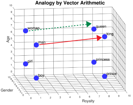
4.3.4 Vector Arithmetic to Solve Analogies

One of the amazing things we can do with feature vectors is solve word analogy problems. An analogy expresses the relationship between similar concepts. Consider this sentence, “man is to king as woman is to _____.” To arrive at an answer, we perform a multi-step calculation. First, we calculate “king” – “man” by subtracting each number in the “man” vector from its partner in the “king” vector. The calculation is (1 – 1), (8 – 7), (8 – 0), resulting in [0, 1, 8]. Then, we add this vector to the one for “women.” The calculation is (0 + 9), (1 + 7), (8 + 0), resulting in [9, 8, 8]. Finally, we look for a word close to that last vector’s coordinates. Is there one? Yes, the word “queen” is nearby!

We can also do this calculation graphically. First, we draw an arrow from “man” to “king.” This is the Euclidean distance between these two words. Next, we take this arrow – keeping the same direction and length – and add it to “woman.” Finally, we see that the “queen” is close by.

4.3.5 Word Embeddings

A 3-dimensional space works well when working with a small set of words. But what if we want to add more words like “cucumber,” “smiled,” or “honesty”? Clearly, we will need a much larger number of semantic features. A semantic feature space of four, five, or even six dimensions can probably accommodate the three new words just mentioned. But what if we want to represent all the entries in a typical 50,000-word English dictionary? Such an undertaking would require us to create hundreds of new features. Think about all that work! Not only will we have to design the features, but we’ll have to assign accurate coordinates to each word as well. This kind of work is impossible for humans to do as it requires one to visualize high-dimensional spaces, far beyond the 3-dimensional world we live in. Is there a way to do this?

Fortunately, large language models (LLMs) can construct these high-dimensional spaces for us. An LLM is a special kind of neural network designed to generate word embeddings. As with any neural network, the first task is to collect a massive amount of data, text in this case. Using that data, we then train the model. During training, an LLM discovers statistical relationships between words that occur together. Those data patterns, in turn, inform how the model positions each word in a semantic feature space. These word representations are called word embeddings. Word embeddings come in various sizes, but a typical embedding has 300 dimensions. That is, the model represents each word with 300 unique numbers.

The figure below shows the embedding vectors for six words in the Carnegie-Mellon Word Embedding Demo. And because this embedding has 300 dimensions, each vector in it has 300 numbers, with values ranging from -0.2 to +0.2. The words “uncle,” “boy,” and “he” are male terms, while “aunt,” “girl,” and “she” are female. On the left, dimension 126 has been magnified. This element appears to correlate with gender as it has slightly positive values (tan/orange) for the male terms and slightly negative values (blue/gray) for the female ones.

A word embedding like the one pictured here is incredibly useful. With it, a model can make sense of analogies, plurals (“hand” is to “hands” as “foot” is to “feet”), past tense (“sing” is to “sang” as “eat” is to “ate”), comparisons (“big” is to “small” as “fast” is to “slow”), and even map countries to their capitals (“France” is to “Paris” as “England” is to “London”).

Word embeddings enable transformers such as ChatGPT or Google’s BERT to figure out what a sentence or entire paragraph says. The transformer architecture is relatively new, introduced in a 2017 article: Attention is All You Need. Although a full examination of transformer architecture is beyond this article’s scope, word embeddings give these models their superpowers, including the ability to generate text in response to prompts.

Also, note that LLMs generate text in a completely different way from humans. The model understands nothing. The process is purely statistical. Given a string of words, transformers like ChatGPT use the context of the input text to compute the probabilities of possible next words. That is, the model creates a probability distribution of all the words in its vocabulary, with one probability for each word in its training dataset. That probability calculation considers the immediate context – revealed by an attention mechanism – and the relationships between words learned during model training. “The temperature parameter controls the randomness of an LLM’s output. A higher temperature produces more creative and imaginative text while a lower temperature results in more accurate and factual text.” ^[4]