6 Retrieval Augmented Generation (RAG) Systems

6.1 Introduction

Retrieval augmented generation (RAG) systems are a recent development, making an initial appearance in 2020 after an article was published by investigators at Facebook’s AI Research group.  But why was a new kind of generative AI needed?  The answer is that organizations, businesses primarily, needed a way to create customer service ChatBots easily.  Business ChatBots, though, require a backend model trained on custom, typically proprietary, data.  A RAG system solves this problem.  Before RAG, the standard approach was to partly retrain a large language model in a process called fine-tuning.  With fine-tuning, a model’s parameters, also called weights, are adjusted as it’s retrained on custom data.  Fine-tuning is a practical yet somewhat fussy process, requiring a certain level of technical expertise.

6.2 Anatomy of a RAG System

RAG systems take a much different approach to custom data.  Rather than adjust a model’s existing parameters (what it has learned already), RAG systems augment a model’s knowledge.

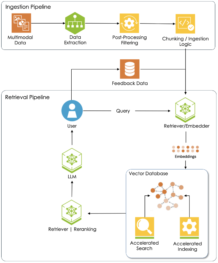
6.2.1 The Ingestion Pipeline

Let’s step through Figure 6.1.  The first step in the ingestion pipeline is to curate a custom dataset of documents that reflect a scholar’s specific research interest or project.  Most documents are multimodal.  That is, they feature texts, images, graphics, even audio and video clips.  Each format type needs to be extracted from the underlying document because AI processing workflows differ for each.   In fact, most AI models are designed to work with just one type of data.  Take, for instance, the convolutional neural network or CNN.  The architecture of this model is custom built for image datasets, specifically recognition tasks.  Transformers, on the other hand, excel at finding meaning in a document set while other models specialize in audio or video processing.  Once the text, images, and other formats have been isolated during data extraction, the post-processing step is where data gets scrubbed.  Consider this case-study:

The final step of the ingestion pipeline is chunking / ingestion logic.  Each embedder has specific limits to the amount of data it can process in each ingestion cycle.  Chunking is the process of breaking down large documents into smaller, more manageable segments or “chunks”.  These are then fed to an embedder that converts them into embeddings.  Those embeddings, in turn, are stored in a vector database such as Milvus or Pinecone.  Vector databases, as explained in section 6.3, are specially designed to store embeddings and facilitate fast search and retrieval operations.

All the documents in a custom dataset are first processed through an ingestion pipeline like the one presented here before the RAG retrieval pipeline is fully activated.  After that happens, the system requires continual monitoring and occasional updating.

6.2.2 The Retrieval Pipeline

The whole point of a RAG system is to allow a scholar to have a “conversation” with a specific dataset of interest to them.  That happens once embeddings for all the documents in the corpus have been generated and stored in a vector database.  To initiate a conversation, the user prompts the system with a question or request, just as they would with any other LLM.  Next, their query is sent to the embedder which converts it into an embedding.  (Keep in mind that the language of AI is numbers.)  With that, an algorithm then searches the vector database for embeddings that have similar meanings.  Matches are ordered by a retriever/ranker and then handed off to an LLM which composes a reply to the user.  The job of the ranker is to ensure that the model has the best content available to do its job.  Most RAG systems can be configured to only use content from the curated document dataset, ignoring knowledge stored in the large language model.  This ensures that model responses are dataset specific and possible “noise” excluded.  Take the case of a prompt about Renaissance Venice.  The scholar, in this case, seeks a historically accurate reply that only uses content from a curated dataset, untainted by LLM knowledge of the modern city and its concerns.

And lastly, many RAG systems allow users to provide feedback to the model.  This information is used to fine-tune the system, making it more accurate and less prone to hallucinations.

6.3 Vector Databases

Let’s begin our exploration of vector databases with a quick review.  An embedder is a computational model that converts images, text, or sound files into vector representations called embeddings.  A vector is just a list of numbers.  More specifically, word embedders convert text into numerical representations called word embeddings.  Some popular word embedders include Word2Vec, GloVe, and FastText.  Bert and GPT are also well liked, being two contextual models valued for their ability to generate context sensitive embeddings.  In this article, our focus is primarily on word embeddings.

Interestingly, embeddings can be generated for just about any digital object.  Here we see three embeddings: one for an image, a second for a sentence, and a third for a sound recording.

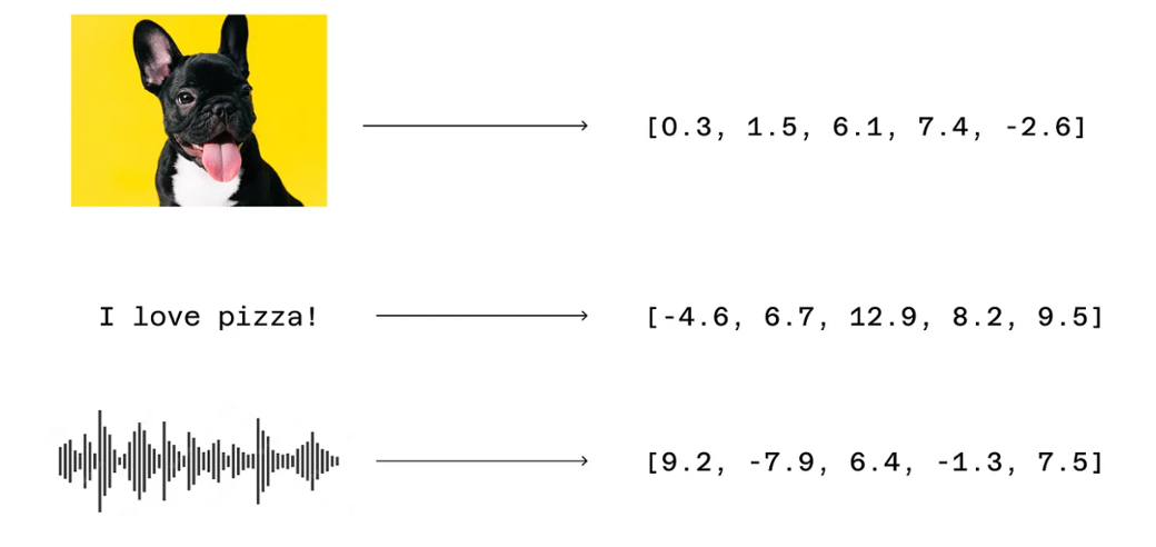
Most word embeddings are high dimensional.  That is, they contain more than one number, often hundreds or even thousands of numbers.  Computer scientists say that an embedding of two numbers is two dimensional, an embedding of three numbers is three dimensional, an embedding of four numbers is four dimensional, and so on.  Here are three examples.

Fortunately, humans don’t have to create these high dimensional embeddings.  The AI models learn them while being trained.  All these numbers make no sense to humans, but they do for the machine.  As Raj Pulapakura writes, “Embeddings are like the five senses for machines, a portal through which they can comprehend the real world, in a language (numbers) they understand.”  What makes word embeddings so powerful is that they can represent the meaning of a text in a way that makes sense to large language models (LLM).

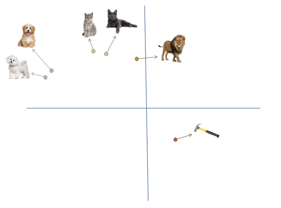
As shown here, an embedder has discovered relationships between the content it trained on, positioning similar items nearer to each other.  The two cats lie close to each other as do the two dogs, but both groups are at a distance from the inanimate hammer.  Now when we say items are similar, what we mean is that their embeddings are alike, their vectors analogous.

Similarity or closeness can be measured in many ways, including cosine distance, dot product, and Euclidean distance.  A small distance between embeddings is an indicator of similarity.  AI models can do amazing things with these numbers – identify and classify images or make sense of written documents like humans do.

The process of generating embeddings is shown in Figure xx.  We start with a document corpus and feed the text incrementally to an embedder in a process called chunking.  During chunking, a document is divided into discrete blocks of text and fed to the embedder one at a time.  The size of those chunks is specific to each embedder.  The model then processes each chunk and generates embeddings for all of the data chunks in a document corpus.

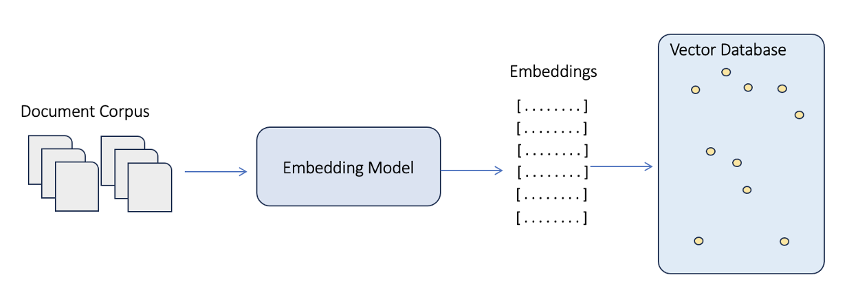
Once all the embeddings for a corpus have been generated, we now need to store them somewhere.  The logical answer is a database management system.  Relational databases are one possibility.  The technology is proven, having first penetrated many corporate IT departments about 35 years ago.  Postgres, for example, has a distinguished pedigree as a relational database.  It now offers the pgvector extension to store and retrieve embeddings.  Embeddings, however, are a unique kind of data, calling for a solution that delivers fast retrieval and efficient similarity search (a topic we discuss next) of high-dimensional data.  Relational databases use indexes to support efficient retrieval operations.

Even though a tried and true solution existed, it became increasingly evident that this new type of data required a new type of database.  Enter the vector database.  Vector databases like Milvus and Pinecone are relatively new offerings.  Zilliz, for example, was released Milvus in 2019.  Vector databases represent a fundamental rethink of data storage technology, a specific response to the increasing demands of advanced AI systems.  They were designed and built from the ground up to handle vector data in all its unique manifestations.

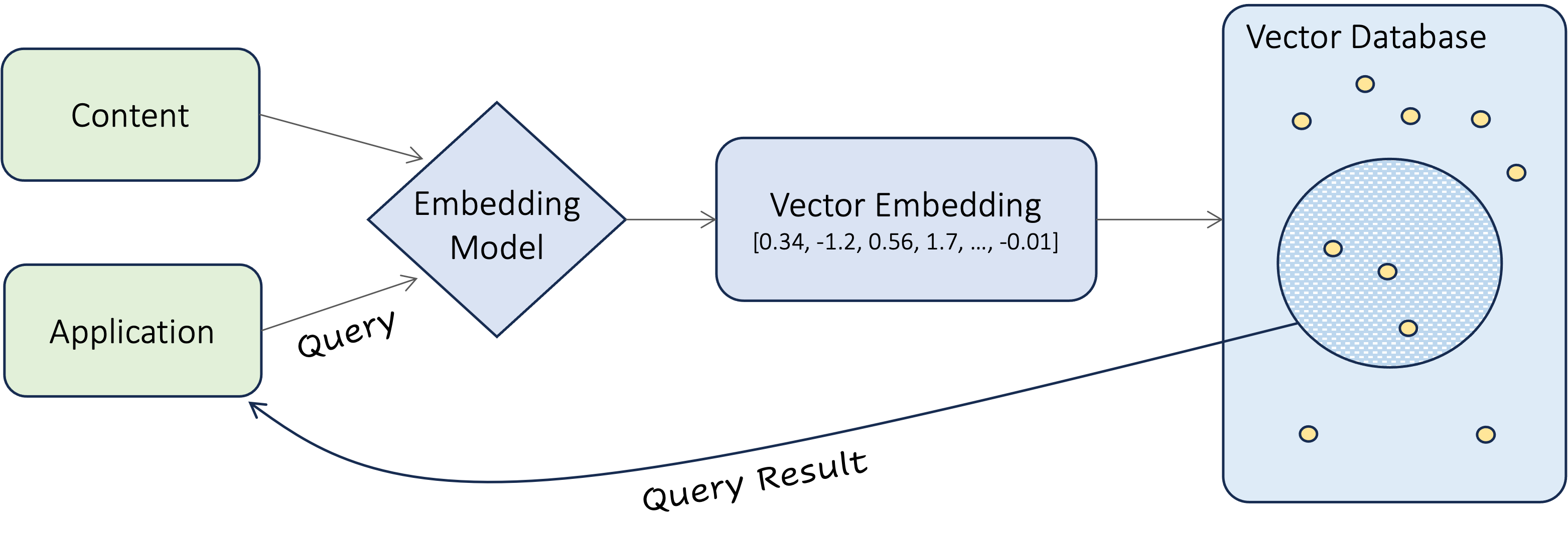
Before we dive into the details of vector search, let’s zoom out and take a look at the entire system.  As we’ve already discussed the process of inserting embeddings into a vector database, we’ll focus our attention on the application data flow in Figure xx.  Here a software application of some sort provides a friendly interface where users enter their search term(s).  The query is then passed to the embedder which converts it into an embedding.  The database then executes a similarity search, comparing the query embedding against all the embeddings stored in it.

But what exactly is a similarity search?  At his Medium site, Pavan Belagatti describes similarity or vector search with a simple illustration.  He writes:

Imagine you have a big box of colorful crayons, and each crayon is a different color. A vector database is like a magical sorting machine that helps you find crayons that are similar in color really fast. When you want a crayon that looks like your favorite blue one, you put in a picture of it, and the machine quickly looks through all the crayons. It finds the ones that are closest in color to your blue crayon and shows them to you. This way, you can easily pick out the crayons you want without searching the whole box!

Essentially, what a vector search algorithm does is find those crayons (embeddings) that are closest in color to your query embedding.  Closeness, as we’ve already noted, can be calculated in a variety of ways:  cosine distance, dot product, or Euclidean distance.  These three work well for small vector databases.  But for large databases storing millions of embeddings with hundreds or even thousands of dimensions, other algorithms such as Locality-Sensitive Hashing (LSH) are faster.  This is an evolving area of research, and technical details of these efforts can be found elsewhere.

Although we do not present those details here, vector databases typically provide a distance score for each item retrieved.  This number is an estimate of semantic closeness between the document retrieved and the user’s search query.  In figure 6.8, a distance score is shown in blue. Higher numbers indicate greater semantic similarity and therefore smaller distances.